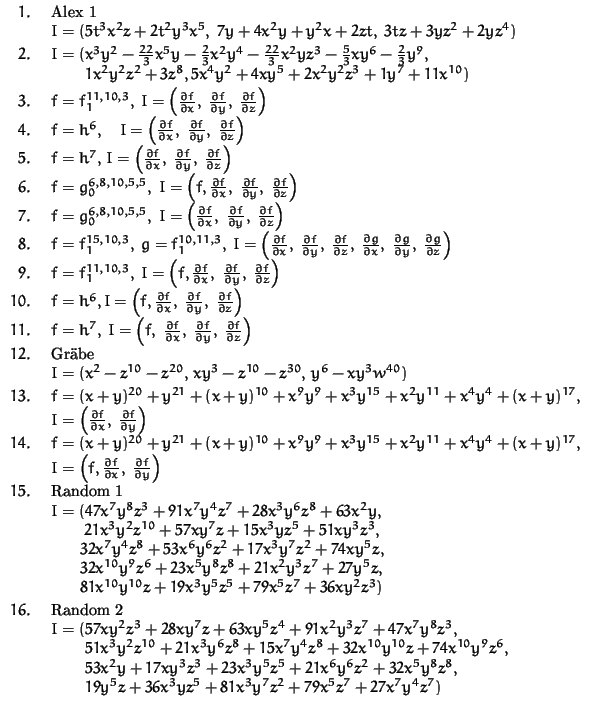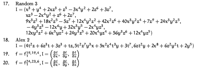
Let

Examples:


Options:
The ordering of the variables is
t, x, y, z, w, the computations were done
in characteristic 32003.
Lazard stands for the algorithm ``Lazard'' and Mora for the
algorithm ``Standard basis'' with NFMora, cf. Chapter 1.
The columns have the following meaning:
We used
The symbol ``#'' indicates usage of more than 120 megabyte and ``-'' indicates that this option makes no sense.
The time is given in seconds (up to one decimal place).
The time 0 indicates less than
0.05 seconds.
Compare the table on the next page.
| MAC | SING | -- | mP | su/mP | suC/mP | su | fHC | ecartM | lex | d(lex) | ||
| 1 | 2 | 3 | 4 | 5 | 6 | 7 | 8 | 9 | w | 10 | 11 | |
| 1 | 53 | 35.7 | 27.9 | 28.2 | 27.6 | # | 27.9 | - | 0 | (5, 2, 2, 1) | 0 | 0 |
2 |
21 | 12.9 | 419.8 | 9.9 | 9.3 | 9.5 | 289.6 | 0 | 1.0 | (95, 94, 63) | 0.5 | 1.1 |
3 |
20 | 13.6 | 4.3 | 8.6 | 8.4 | 6.2 | 4.4 | 0.2 | 0.9 | (86, 67, 51) | 0.4 | 1.18 |
4 |
2 | 1.6 | 6.9 | 3.5 | 3.4 | 1.4 | 6.6 | 0 | 1.4 | *(4, 3, 3) | 0.9 | 0.4 |
5 |
2 | 0.8 | 2.8 | 2.8 | 2.7 | 2.5 | 2.7 | 0.5 | 1.4 | *(5, 3, 3) | 2.1 | 1.3 |
6 |
12 | 7.3 | 26.5 | 4.5 | 4.5 | 4.7 | 26.9 | 0 | 1.0 | (16, 8, 5) | 0 | 0.1 |
7 |
6 | 3.5 | 21.1 | 2.2 | 2.2 | 2.5 | 20.6 | 0.4 | 0 | (16, 8, 5) | 0.1 | 1.7 |
8 |
3 | 1.9 | 0 | 0 | 0 | 0 | 0 | 0 | 0.1 | (60, 55, 64) | 0.1 | 0.4 |
9 |
7 | 4.1 | 6.8 | 3.0 | 3.1 | 2.2 | 7.4 | 0 | 6.2 | (10, 11, 7) | 0.2 | 0.3 |
10 |
2 | 1.3 | 4.3 | 4.2 | 4.2 | 2.0 | 6.3 | 0 | 3.0 | *(5, 4, 4) | 0.3 | 0.2 |
11 |
1 | 0.7 | 4.9 | 4.6 | 4.4 | 2.2 | 4.9 | 0.3 | 3.5 | *(5, 4, 4) | 0.3 | 0.6 |
12 |
4 | 1.2 | # | # | 559.5 | 0.3 | # | - | 0 | (20, 20, 2, 1) | 0 | 0 |
13 |
237 | 84.2 | # | 43.4 | 44.1 | 87.4 | 0 | 1.0 | *(4, 3) | 0 | 0 | |
14 |
33 | 14.2 | 2520.8 | 56.7 | 53.4 | 44.3 | 2438.7 | 0 | 7.7 | *(4, 3) | 0.2 | 0.1 |
15 |
2405 | 1480.4 | 0 | 0 | 0 | 0 | 0 | - | 0 | (47, 64, 62) | 0 | 0 |
16 |
6156 | 4113.7 | # | # | # | # | # | - | # | (35, 38, 61) | 0 | 0 |
17 |
5 | 3.3 | 14.7 | 1.6 | 1.6 | 1.3 | 15.0 | 0 | 1.2 | (2, 3, 2) | 0.1 | 0 |
18 |
4383 | 3838.4 | 0.6 | 0.1 | 0.1 | # | 0.5 | - | 0.3 | (32, 12, 19, 13) | 0 | # |
19 |
17641 | 9190.2 | # | 2205.2 | 2033.6 | 2253.6 | # | 2.2 | 92.9 | *(4, 3, 2) | 6.3 | 8.7 |
20 |
83965 | 50265.5 | # | 32421.8 | 33447.3 | 8855.7 | # | 315.0 | # | (76, 65, 47) | 135.9 | 816.6 |
Conclusions: (for the case
Loc;SPMlt; K[x] = K[x](x))
The above examples and many more tests which have not been documented show the
following pattern:
These are general principles which have proved useful. Moreover, in SINGULAR the options can be combined by the user. Of course, there are always special examples with different behaviour. For example, in example 12 sugarCrit + morePairs is very good, but in example 1 it is the worst option. There is no option which is universally the best. The standard basis algorithm is extremely sensitive to the choice of the strategy, in the local case ( Loc;SPMlt; K[x] = K[x](x)) even more than in the inhomogeneous Buchberger case. The homogeneous Buchberger case, on the contrary, is much less sensitive to the choice of the strategy and is very stable. This explains why Lazard's method did always succeed, but on average is much slower. The ecartMethod (in connection with HC) seems to be by far the best. But we did not succeed in finding a good ecart vector for example 16. Here lex together with d(lex) is the best (less than 0.1 seconds). The conclusion is that at the moment a system has to offer several strategies, a default one which is good in most cases, but also gives the user the possibility of another choice.
Moreover, for computations in characterstic zero or over algebraic extensions the growth of the coefficients has to be taken into account in the strategies.
We tried to compare the timings also with Faugère's GB, but GB neither offers the ordering used in Columns 1 and 2 nor the tangent cone orderings used in the remaining columns. Testing several homogeneous examples in positive characteristic with degrevlex ordering showed, however, that SINGULAR is about 1.4 times faster than GB (on a Sparc2 and on an IBM RS/6000).